Noise Studio is a post-processing program that can perform sound analyses in compliance with current Italian and European Community norms. The analysis functions are grouped in software modules that can be enabled using a licence.
The analysis environment gives several display functions (as a table or graphically) of the different sound measurements and processed results. All graphs and tables can be exported to other applications in the Windows® environment. The analysed data and results can usually be stored as projects, together with other documents, so as to allow future checks and analyses.
You can process the data downloaded from the sound level meter memory, and the data captured directly by the PC's memory using the NoiseStudio - Monitor Module program.
The Monitor module allows you to manage the HD2010
and HD2110 sound level meters from your PC. There are two methods of connecting
the instrument to the PC: direct connection to the computer via the serial
port or remote connection via modem and telephone line. Thanks to the
modem connection, the sound level meter can be fully controlled remotely
and the acquired data sent to the PC and displayed on the monitor in real
time. Furthermore, thanks to the Scheduler feature, the acquisition intervals
specifying the start and stop moments and the intermediate pauses can
be scheduled. Using the Scheduler it is also possible to perform electric
calibrations before and after each measurement series.
Among their other characteristics, the configuration parameters can be
set, such as displaying the data as a table or graphically and saving
them on file, of printing the data and exporting them in an Excel®
or text format, of copying the contents of the main window and pasting
it into another application as a graph or text, of updating the instrument
firmware,…
The Monitor module fully manages the HD2010 and HD2110 sound level meters using direct connection through a serial cable or via a telephone line with the use of two modems. All the functions described in this manual remain valid for both the direct serial connection and for the remote connection via modem except for the sound level meter firmware update which is only available through the direct connection.
The two instrument's connection modes are described in detail below: direct serial connection and remote connection.
1) Connect the sound level meter to a free serial port on the PC (COM1, COM2,...) using the special cable supplied with the instrument (HD2110/CSNM).
2) Start the application by double clicking on the application icon on the desktop, or select the Monitor item in the DeltaOhm folder on the Start menu.
3) Turn on the instrument and wait for the start-up routine to finish.
4) Set the baud rate on the sound level meter to 38400 baud or 57600 baud (Menu >> General >> Input/Output >> RS232BaudRate).
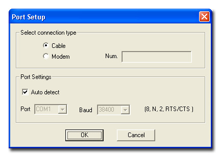
5) In the Monitor module, select the menu item Options >> Port Setting. The serial port configuration window opens:
Select the Cable type of connection and the Autodetect item, as shown in the figure above. To confirm, click the OK button.
|
|
6) Press the Connect button or select the command Instrument >> Connect: the application will automatically search and connect to the serial port to which the instrument is connected. |
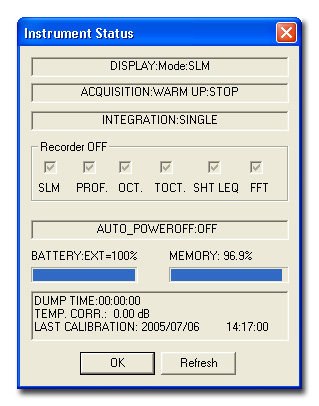
After successful connection, the page showing the firmware version and the instrument's serial number will appear, and after this, the page that summarizes its current status:
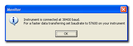
If the baud rate value set on the instrument is not the maximum available (equal to 57600 baud), a window will pop up prompting you to increase this value (See also the paragraph Trouble Shooting).
If the connection is successful, the following symbol will appear to the lower right:
![]()
A failed connection will be indicated by the following symbol:
![]()
If the application is unable to connect to the instrument please refer to the following section in this manual: Trouble Shooting.
Note: do not use the instrument keyboard until the connection with the PC is enabled or the scheduler has been set so that possible functioning conflicts will be avoided. Before using the instrument again, disconnect it by pressing Disconnect.
![]()
When the instrument is not connected to the application the status bar shows the following symbol:
![]()
The remote connection requires the use of two modems: the first connects the sound level meter to the telephone line, the second connects the PC to the telephone line.
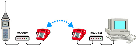
While the modem connecting the PC to the telephone line does not have to conform to specific requirements, except to be Hayes© compatible, the sound level meter itself must be used to configure the modem used to connect the PC and the meter, as any improper messages must not be inserted during the delicate data transfer phase. Delta Ohm s.r.l. tested three suitable modems for the connection:
Multitech MT2834ZDX
Digicom SNM49
Digicom Botticelli
Other types of modem could be used but, due to the variety of products available on the market, assistance is not provided for the connection to modems other than those listed.
1) Configuration of the modem connected to the sound level meter
The modem connected to the sound level meter must be configured before being used for the data transfer. The configuration is completely and automatically performed by the sound level meter itself after the following steps have been performed.
A. Connect the modem to the sound level meter using the HD2110/CSM cable. Make sure you are using this specific cable for the modem and not the general serial HD2110/CSNM cable supplied with the sound level meter.
B. Connect the modem to the telephone line and to the power line.
C. Turn the modem on.
D. Turn the sound level meter on.
E. Set the sound level meter communication speed to at least 38400 baud by accessing the parameter MENU >> General >> Input/Output >> RS232 Baud Rate.
F. Set the parameter on the sound level meter MENU >> General >> Input/Output >> RS232Prot. on the item MODEM and press ENTER to confirm.
The instrument automatically configures the modem. The configuration is confirmed at the end of the set up process by the message "Modem Configured."
In case of failure the sound level meter will automatically return in CABLE mode and the message "Configuration failed!" will appear.
Possible under voltages on the modem do not create problems as the configuration
is memorized and automatically loaded on turning it on.
2) Connect the second modem to the PC and to the telephone
line.
Please see the user's manual supplied with the modem for the modem's installation
and configuration.
3) Start the application by double clicking on the application icon on the desktop, or select the Monitor item in the DeltaOhm folder on the Start menu.
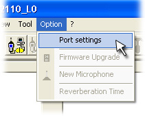
4) Select the menu item Option >> Port settings. The serial port communication setting page will open:
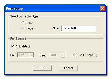
Select the Modem item for the type of connection, and in the Num. box enter the telephone number of the line trough which the second modem is connected to the sound level meter. The Auto detect item must remain selected. The Auto detect item must only be deselected for modems working at a fixed baud rate, and the baud rate value of the modem must be set manually.
|
|
5) Press the Connect button or select the command Instrument >> Connect: the application will activate communication with the modem and, via the telephone line, will connect to the sound level meter. |
After successful connection, the page showing the firmware version and the instrument's serial number will appear, and after this, the page that summarizes its current status:
If the connection is successful, the following symbol will appear to the lower right:
![]()
The symbol will remain until the remote connection via modem is activated.
A failed connection will be indicated by the following symbol:
![]()
If the application is unable to connect to the instrument please refer to the following section in this manual: Trouble Shooting.
Note: do not use the instrument keyboard until the connection with the PC is enabled or the scheduler has been set so that possible functioning conflicts will be avoided. Before using the instrument again, disconnect it by pressing Disconnect and remove the serial cable.
![]()
When the instrument is not connected to the application the status bar shows the following symbol:
![]()
The steps to set the instrument up, and start and stop recording with
Monitor module are now outlined.
Perform the following procedure:
| |
Set up the connection between the sound level meter and the PC as reported in chapter Monitor module Start up. |
Launch the Monitor module and click on Connect. |
|
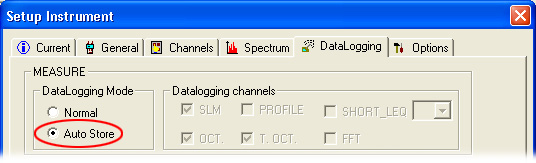
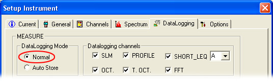
Click on the Setup button and select the Datalogging tab: |
|
 |
|
Select the DataLogging Mode: NORMAL or AUTO-STORE. Select the Normal mode and the channels to be recorded in the DataLogging
Channels or the Auto-Store mode.
|
|
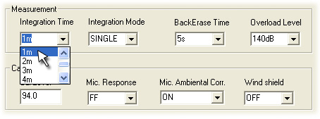
Select the General tab and set the desired Integration Time: at the end of the time set, the sound level meter ends the recording automatically. |
|
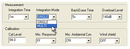
Select the Integration Mode: SINGLE or MULTI
|
|
Set the other parameters as needed (See Instrument Setup) and confirm with APPLY ALL. |
|
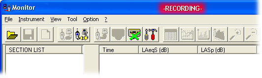
| To start recording, press Start Recording: the title bar of Monitor will signal that the sound level meter is recording using the flashing writing: RECORDING. |
|
| |
|
| To end the recording function, press Stop Recording. |
Monitor module displays in real time the measurements acquired by the sound level meter in both table and graphic form and when the measurement session ends, it can save them to a file so that the data can be reviewed later. Furthermore, the Monitor command works with both the direct and the remote connection.
| |
Set up the connection between the sound level meter and the PC as reported in chapter Monitor module Start up. |
When the connection to the sound level meter is working, set the channel to be monitored (integration time, variables to be integrated, ...) by selecting the Instrument Setup command. |
|
| Click on the Monitor button or select the menu item Instrument >> Monitor. |
|
The application will find the current setup status of the instrument and will open the following window for selection of the measurement channel. |
|
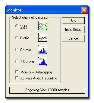 |
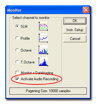
Select the channel to monitor: SLM, Profile, octave or third octave spectrum.
Enable the "Monitor+Datalogging" item to monitor the selected data through PC and at the same time start the sound level meter datalogging function: the recorded parameters may be different from the monitored ones.
Select the "Activate Audio Recording" item to record the sound on which the measurements are carried out. The sound is recorded, through the PC audio card, in a "wav" file (for further details click here ).
Select the size of the single data page: the latter can vary from 200 to 10000 samples. With computers having limited hardware resources, it is recommended to use a limited number of samples to speed up processing times.
To start the Monitor, click on OK.
If the instrument is not in STOP mode, a warning message prompting the termination of the acquisition or its continuation will pop up. Pressing YES before starting the Monitor function, ends the acquisition of the integrated measurements. Pressing NO resets the integrated measurements.
The function continues until the Monitor button is clicked again or the menu item Instrument >> Monitor is selected.
The acquired data can be saved on file using the File >> Save as… command or by using the corresponding button.
Disconnect the instrument at the end by pressing Disconnect.
The Monitor module controls the recording of the sound on which the measurements are carried out, through the PC audio card. The sound is recorded on your PC hard disk in a "wav" file.
This function proves useful as a reminder, to listen to a sound leading to certain results or in case the measurements are performed without operator.
The audio recording is synchronous with the data recording on the sound level meter: an indicator will show you the sound corresponding to the data displayed on the graph.
The signal comes from the sound level meter LINE output...
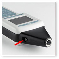
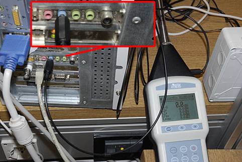
...and it is sent to the LINE IN (or if not available, to the MIC IN
) of your PC audio card.
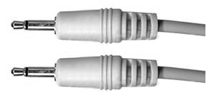
A shielded cable with 3.5mm Mono Jack plugs is used for the connection.
The "Activate Audio Recording" command is available in the Monitor and Scheduler functions setup:
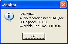
As soon as the "Activate Audio Recording" command is selected, a window pops up showing the space available in your hard disk:
The audio card setup window will then appear.
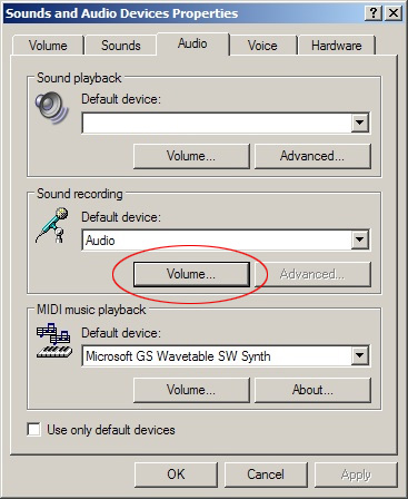
Enter the Volume section and activate only the Line In channel (or Microphone).
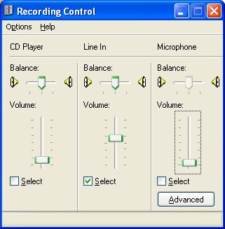
The main window will appear:
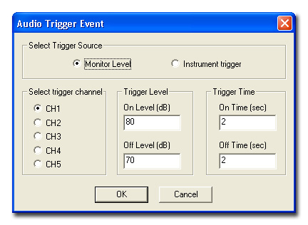
The audio recording starts and ends with the trigger signal. This signal can be the exact value of one SLM channel level (Monitor Level) or, if the "Advanced Analyzer " option is installed, a signal generated by the "Event Trigger " (for further details please look at HD2110 manual).
Monitor Level
Select the channel to use as a trigger (Select trigger channel),
the On Level and Off Level, the minimum On Time
and Off Time.
Notes:
Instrument Trigger
The trigger linked to the "Event Trigger" function does not
require further adjustment (please refer to the Datalogging
window in the instrument setup).
Press OK to confirm and start the Monitor or Scheduler function.
When the recording function ends, the results are shown on the graph: all the events accompanied by audio recording are marked with dotted lines and Ev.1, Ev.2,...
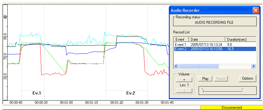
By saving the results you will create a folder with the same name as the file: inside you will find the file with a "dr5" extension as well as all the audio recordings.
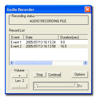
The recording and view of results are handled by the following window which opens automatically when there are audio recordings:
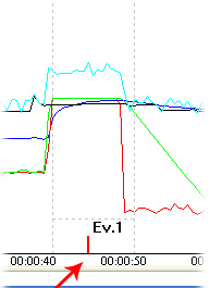
In the PLAY mode of a recorded event, a vertical red line on the graph shows the point that you are playing back:
The Monitor module page will appear as follows:
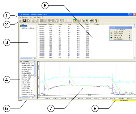
The following functional areas can be seen:
1. Main Menu: it collects the menu
items.
2. Command Bar: a set of icons corresponding
to the main commands of the application.
3. Pages: list of the downloaded pages.
4. Instrument Parameters: resumes the current settings of the instrument
5. Status Bar: provides the information
on the current command.
6. Data Window: displays the current data in tabular form.
7. Graphic Window: graphic display of current data.
8. Connection status of the serial port.
The data arriving from the instrument can either be displayed as a table or graphically. For spectrum analysis a three-dimensional graph is also available.
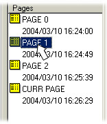
In the column on the upper right (PAGES) the data pages acquired
by the Monitor function are displayed.
To select a page you only need to use the left button of the mouse to
click on the name of the PAGE.
The type of data that can be monitored consists of one of the following items:
SLM
PROFILE
OCTAVE
TOCTAVE
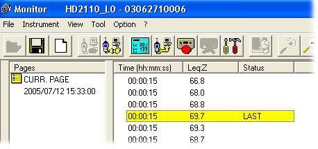
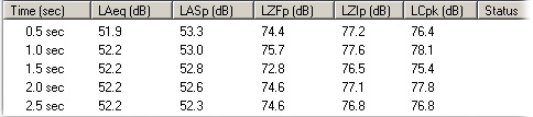
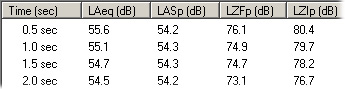
The SLM item shows the Sound Level Meter parameters, acquired at a fixed rate of 0.5 seconds as reported in the sample table below.
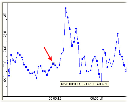
The graphic display is shown in the following figure:
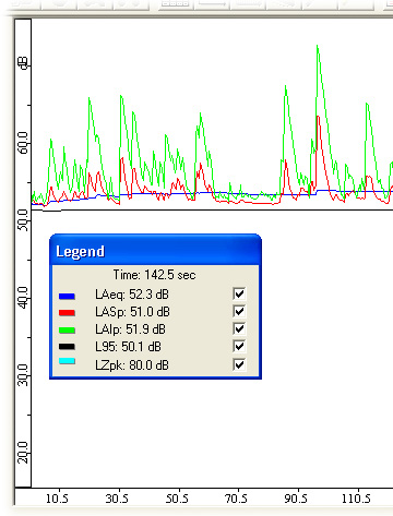
The legend on the graph provides the value of the variables corresponding
to the mouse indicator position on the time axis.
Note: the possibility of excluding some parameters on the display is only
active after the Monitor function has been closed.
The data table is continuously updated with new lines as new samples
are acquired. To block the upward movement of the lines in order to analyze
the table before completion of the page, double click on any line. The
table freezes yet the new samples are still being added to the page. To
restore the normal display mode right click on the table.
Note: this operation does not stop the data acquisition but only the display
of the data.
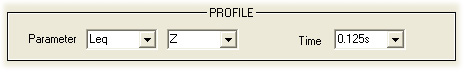
The PROFILE item shows the History Profile parameter acquired within the sampling interval equal to the Profile Time. It is displayed as a table and as a continuous graph.
If the spectrum analysis is set as multi-spectrum (MLT, MAX or MIN), OCTAVE and TOCTAVE display a sequence of octave or third octave spectra acquired in a time interval equal to the Spectrum Profile Time. Each spectrum memorized will appear on the monitor in sequence: as a data table and contemporaneously as a histogram. To analyse the entire set of spectra you have two tools: the Spectrum Navigator and the 3D graph.
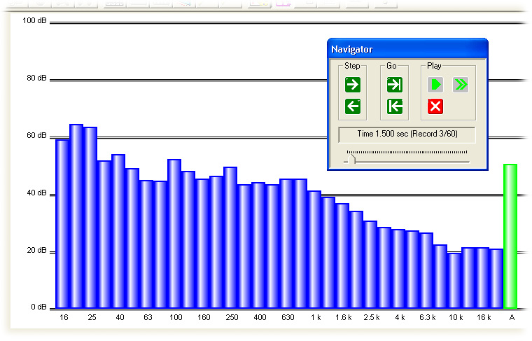
The Spectrum Navigator only appears after having closed a monitor session and saved the file.
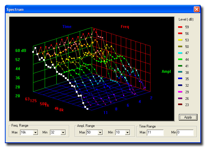
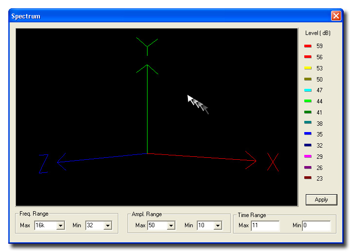
The contemporaneous display of the entire set of spectra requires a three-dimensional graph that shows the following three variables: central frequency of the filters, sound level and progressive number of the samples. The function can be activated during the monitoring of octave and third octave spectra.
|
To enable the three-dimensional graph press View 3D Graph or select the menu item View >> View 3D Graph. |
The graph is displayed in a separate page that opens automatically.
The graph reports the profiles of the spectra being acquired according to the frequency (X axis), width (Y axis) and progressive number of samples (Z axis). The extreme limits of the three variables are initially chosen to improve the display of the overall graph: by operating on the drop down menu in the lower part of the page, it is possible to modify the graph display. The changes only take effect if you intervene on all three ranges: by selecting manual ranges both for frequency and for width the time range can also be modified. Only now can the APPLY button be pressed to effect the changes.
The 3D graph can be rotated in all three directions by clicking directly on it with the mouse. Moving the mouse pointer on the black background window and keeping the left button pressed, the three axes of the graph are highlighted. By dragging with the mouse, again without releasing the button, the axis can be rotated freely. When you let go of the button the graph is altered.
| |
The icon on the left changes the time reference for the data displayed, both for a table or graphically: it alternates an absolute (actual date and time of acquisition) and a relative (time passed after the Start command that begins from the instant 0) time reference. |
The function can also be enabled from the menu selecting View >> View Full Date-Time.
The following figure gives an example of a data table with a relative time reference:
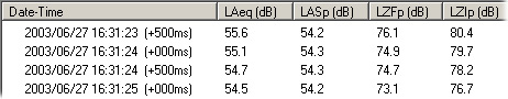
The following figure is the same table with an absolute reference:
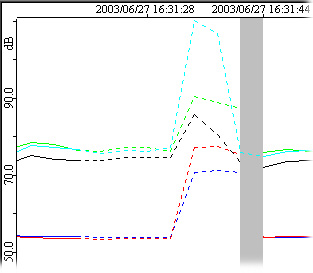
The activation of the absolute time display in the graphs indicates the data acquisition is discontinued due to the use of the PAUSE/CONTINUE function: the data corresponding to the moment when the CONTINUE button is pressed after a pause, is marked by a grey vertical bar.
When in the main window is displayed a graph in modes SLM and History Profile appears, a click with the right button of the mouse opens a menu containing the following commands:
Point marks displays the sampling moments using points on the graph.
View status LAST: when the multiple integration is enabled, a special marker (“Last”) is stored together with the last data recorded before reducing to zero the integrating levels and before beginning a new integration interval.
The command displays a square corresponding to each LAST label on the graph.
Axis applies a dotted grid on the graph.
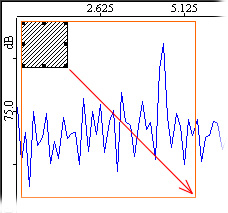
Zoom enlarges a selected area of the graph.
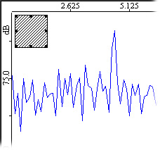
To enlarge a part of the graph, select the Zoom tool. A selection box will appear in the upper left-hand corner:
Press the left button of the mouse over the box and drag it in the graph area to be enlarged. Then use the eight "handles" on the edges to resize the selected area:
Now press the Zoom+ button
To return to the default view press the Zoom- button
Fit… fits the graph dimension in order to cover the entire available height (Height), the entire width (Width) or the entire page (Page).
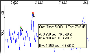
Set Marker A - Set Marker B - Clear Markers : the function Trace Mouse Coordinates shows the difference between two points A and B of the graph: to select the two point, click on the first with the left button of the mouse and then use the right button to select the item Set Marker A; repeat the operation to mark the second point B by selecting the item Set Marker B. The label appearing on the graph will display the sound level difference between the two points:
To remove the two markers, select the Clear Markers command.
If the graph refers to the reverberation time calculation, the label appearing will also show the reverberation time calculated between the two selected points (See the chapter on reverberation time in the DeltaLog5 or DL5Viewer Help).
The Monitor application can perform the drawing the isophonic curves on the third octave spectra, according to ISO 226/1987 and ISO226/2003.
When a third octave spectrum is displayed, the function is enabled through the menu item Tool >> View E.L.Level >> E.L.Level 1987 or Tool >> View E.L.Level >> E.L.Level 2003.
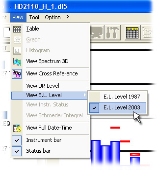
To select an isophonic curve, click on the band corresponding to the particular central frequency: the corresponding isophone with a level equal to the spectrum corresponding to the selected band will be displayed. By confronting the isophone levels with the spectrum levels it is possible to evaluate the audibility of the selected band.

For the bands with central frequencies equal to 16 Hz, 16 kHz and 20 kHz, where the isophonic curves are not defined, or if the level of the selected band is lower than the audible minimum, the isophonic curve of the minimum audibility (MAF) is displayed, as outlined in the following example:
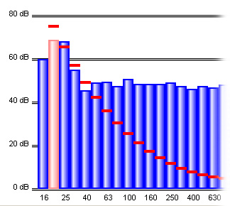
The label appearing when moving the pointer over the spectrum shows the central frequency and the filter level, the isophone value and the difference (delta) between the current isophone and the band level on which the pointer is positioned.
The data displayed as a table can be automatically exported to an Excel spreadsheet by pressing the Export to Excel button.
![]()
In multiple sessions, you can choose to export either only the current spectrum or the set of spectra making up the session:
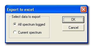
Together with the data, a page with the instrument's parameters is exported.
There is a filter to export the data in text format.
| With the instrument connected, press the Setup button to open the dialog box and set the parameters. |
The window has 6 tabs:
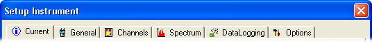
Current: summarizes all current data and instrument settings – this tab cannot be edited by the user.
General: this is divided into 4 sections called General, Input/Output, Measurement and Calibration.
General
The upper part is used to set the date and time of the sound level meter:
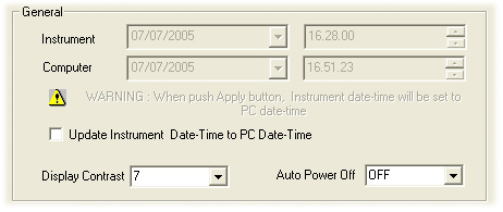
The date and time of the instrument at the moment of the connection with the PC, and date and time of the PC itself, are both reported: selection of the item Update Instrument Date-Time to PC Date-Time, uses the date and time of the PC to update date and time of the instrument. The date and time proposed can be changed by acting directly on the windows labelled Computer.
Display Contrast regulates the display contrast of the instrument: a high value increases the contrast, a low value decreases it.
Auto Power Off enables (ON) or disables (OFF) the automatic shut off of the instrument after the keyboard has been inactive for 5 minutes or more.
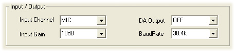
Here you can:
select an entry channel (Input Line = Microphone, Entry Line or Entry Digital Audio). For HD2010 the entry channel can be only a Microphone.
amplification 0 or 10dB for HD2110 and 0 dB to 40 dB with increments of 10 dB for HD2010. Entry amplification can be adjusted to 0 dB or 10 dB also for HD2010 with the option "Extended Range".
enable or disable the Digital Audio output (DA Output) for HD2110.
select the Baud Rate of the serial communication.
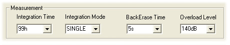
Measurement
Integration Time represents the integration time indicated on the sound level meter as Tint.
Back Erase Time is the back erase time of the acquired samples used to exclude them from the calculation of the integrated parameters. The delete function is not managed.
Overload Level sets the maximum level for the overload signal and is displayed when exceeded.
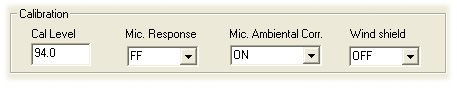
Calibration
The items reported in this part of the tab deal with the calibration of the instrument and the corrections of the measurement.
Cal.Level is the level used to perform the acoustic calibration of the sound level meter: usually the values of 94 or 114 dB are used.
Acoustic Field is the correction of the frequency response of the microphone according to the type of acoustic field: FF means Free Field and RI means Random Incidence.
Mic. Ambiental Corr. is the correction of the microphone sensibility according to the temperature read by the internal sensor. This value is ON by default.
Wind Shield is set to ON when the wind shield is used and you would like to compensate the frequency response of the microphone.
Channels: by using this tab you can select the SLM and History Profile parameters with their relevant weightings.
The sampling interval of the profile is shown near the History Profile parameter.
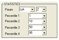
Statistics shows the parameter used for statistical calculations (LFp, Leq or Lpk) with the relevant weighting and, in the lower part of the card, the values corresponding to the Percentile Levels indicated on the sound level meter as L1, L2, L3 and L4.
The so called Percentile Levels indicated on the sound level meter as L1, L2, L3 and L4 are reported in the lower part of the tab.
Dose Integration collects the calculation parameters of the DOSE: Exchange Rate, Dose Threshold and Dose Criterion.
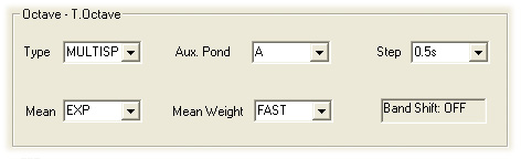
Spectrum resumes the properties of the octave and third octave spectra.
Type is the analysis method: average (AVG) or multi-spectrum (MLT, MIN, MAX).
Mean and Mean Weight represent the type of mean (LIN or EXP) and relevant weight (for the exponential average (EXP) the weight can be FAST or SLOW).
Aux. Pond. is the weighted frequency of the auxiliary wide band channel represented by the vertical bar of the display.
Step reports the integration or sampling time for spectrum analysis with linear average (LIN) or exponential average (EXP).
The item on grey background Band Shift gives the type of spectrum used by the sound level meter: OFF means that the standard set of filters is being used; ON that the sound level meter is using half band shifted filters. The shift from one type to another can only be carried out from the instrument's menu. The acquisition mode of the third octave spectra is not managed.
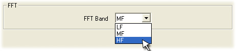
In FFT Band you can select the portion of audio spectrum (LF, MF or HF) where the narrow band analysis is displayed.
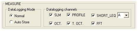
DataLogging is used to enable or disable the channels whose parameters are saved during the recording operation (recording).
Measure
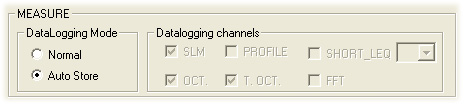
DataLogging Mode can be Normal or Auto Store: the former displays the channels to be recorded in the DataLogging Channels section:
If the DataLogging Mode is set as Auto Store, the channels to be stored will be SLM, octave spectrum and third octave spectrum.
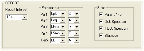
Report
It specifies the parameters corresponding to the report management ("Advanced Analyzer")
Select the interval for storing the reports (Report Interval) and the SLM parameters. In the Store section, enable the items that you want to store.
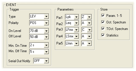
Event
The Event section contains the "Event Trigger " function setup ("Advanced Analyzer"option).
Type: trigger source
Polarity: trigger polarity
On Level and Off Level: trigger On and Off level
Min. On Time and Min. Off Time: minimum duration of the event and stop delay
Serial Out Notify: if enabled (ON), a warning string is sent through the serial interface corresponding to each trigger signal.
Set the items related to the trigger and, if necessary, select SLM parameters. In the Store section, enable the items to store.
Options
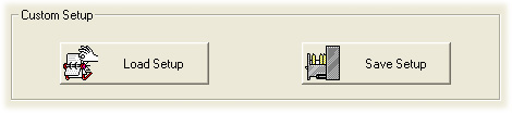
The settings selected in the different Setup tabs can be saved in order
to recover them later: this allows time to be saved and avoids errors
in setting the sound level meter.
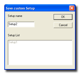
By pressing Save Setup the following window appears for the new setup name to be entered. The list shows the setups in the memory.
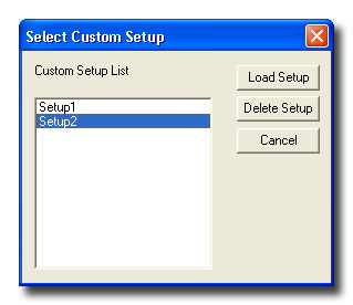
By pressing Load Setup the following window appears:
Select a setup from the list and activate it by pressing Load Setup.
The Delete Setup button deletes the selected setup.
Confirm the settings with the APPLY ALL button or press Cancel.
The scheduler performs the function of planning the Monitor's
and Recording's functions and can be fully configured according to user's
operating requirements. The scheduler is used to set the monitor's scheduled
start and stop dates, the number and duration of any possible pause, the
turning off or not of the sound level meter between two acquisition intervals.
Furthermore, the software can automatically perform an electrical calibration
before or after an acquisition interval or at a certain date. The calibration
can be confirmed or not if the departure detected is above or below a
preset value.
The scheduler function can be activated via both direct connection or
using a remote connection via modem.
The various components of the Scheduler are outlined below.
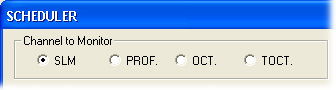
Select the channel to be monitored in Channel to monitor: it is only possible to acquire one channel at a time.
Acquisition Date-Time is used to set the start
date and time (Start Time) and the stop date and time (Stop
Time) for the Monitor;
Acquisition Interval introduces some pauses between the scheduled
start and stop.
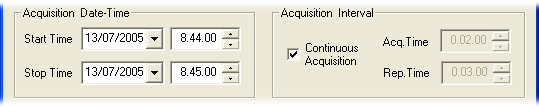
If the item Continuous Acquisition is selected, the monitor proceeds without interruptions, from the Start Time to the Stop Time. Or introduce some pauses, deselect the item and enter the acquisition interval in the Acq.Time and the duration of the repetition in the Rep.Time. The following graph shows what the different items mean.
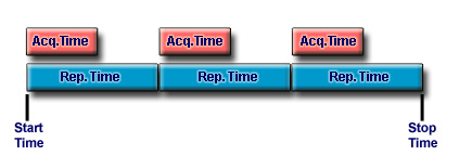
The Stop Time has priority on the acquisition and repetition times therefore the last interval could get cut off before the end by the Stop Time.
In the Instrument section of the scheduler there are these items:
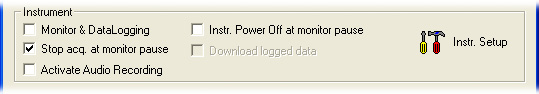
Monitor & DataLogging: when this function is selected, in addition to the transfer to the PC (monitor) of the "Channel to Monitor" selected in "Acquisition Date-Time" , also the channels selected in the menu "Data Logging" of the sound level meter (Instrument Setup) are contemporaneously saved in the instrument's memory (datalogging). Once this item is enabled, you are asked if you want to delete the sound level meter memory to make space for new data (recommended choice). If the item is not selected, the scheduler only enables the monitor.
Download logged data becomes active if the item Monitor & DataLogging is selected. By selecting it, the memorized data are downloaded on the PC at the end of the acquisition (Stop Time).
Stop acquisition at monitor pause: when selected the sound level meter stops after the scheduled monitor period. If this item is not selected the sound level meter will continue to measure eveng during the pauses. This function is valid only if the acquisition intervals are scheduled and allows managing independently the Data Logging and Monitor functions. This function is useful while monitoring the SLM channel, if you wish to reset the integrated parameters at the beginning of each acquisition period. Indeed, when the sound level meter stops, the integrated parameters calculation ends and at the next acquisition, the integrated parameters values will be set to zero.
Instrument Power Off at monitor pause: at monitor pause turns off the sound level meter between two successive acquisitions.
The Instr. Setup button opens the window Instrument Setup allowing setting the sound level meter without exiting the scheduler.
Electric Calibration
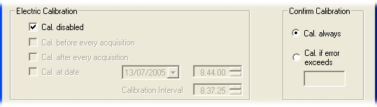
During the monitor electric calibration of the sound level meter can be carried out to detect and/or compensate possible departures. By deselecting the item Cal. disabled, the electric calibration can be selected before (Cal. before acquisition) or after (Cal. after acquisition) each acquisition session. The item Cal. at date allows the date and time when the first calibration needs to be performed to be entered, and using Calibration Interval the time interval before repeating the operation can be entered. These calibrations are performed only during the pauses.
As a final result, the electric calibration gives the difference
between the new calibration value and the one memorized in the sound level
meter.
Selecting the item Cal. always, the calibration data are updated
independently of the departure.
If you wish the calibration to be confirmed only if the difference is
above a certain threshold, select Cal. if error exceeds and enter
the minimum departure that will cause the update of the calibration data.
Complete the set-up and start the scheduler:
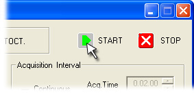
Press STOP to close the scheduler before its end.
The upper part of the page contains the main menu from which all functions offered by the Monitor application can be accessed.
All that is necessary to activate a function is the opening of the drop-down menu where the function is located and its selection with the mouse. According to the context, some menu items are disabled as the function performed is not active: these items are reported in grey.
Each detail and function of the various commands are listed and illustrated in the following pages.
Open
Opens a saved file. The files managed by the application have a DR5.
DR5 is a data file obtained from a monitor
If the instrument is connected to the PC, the Open File command cannot
be used to open a file: you must disconnect first. Clicking on the Open
File button brings the following message up on the screen:
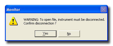
Press Yes to disconnect the instrument and open the file, press No to remain connected.
Save As…
Opens the following window to save the file.
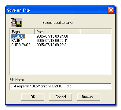
The pages (PAGES) that make up the set
of data are listed in the main window. It is possible to select them all
or only some of the pages to be saved: to select a consecutive group of
pages, click on the first one and then, holding down the Shift,
click on the last. To select a non consecutive group of pages, click on
each one while holding the Ctrl button down.
The Browse button can be used to modify the position of the file, or the
complete path can be typed in the File Name line.
The File Name window shows the name and the position of the file.
The OK button is not activated until at least one page has been selected
for saving.
Export to Excel
Opens Microsoft Excel and exports the currently active data into an Excel
folder. The Microsoft Excel application must be installed on the PC in
order for this feature to be enabled. Up to 30000 samples per time are
exported. For higher quantities you are prompted for the data block to
be exported.
See also the paragraph Exporting Data.
Export as formatted text
Export the currently active data into a text file with the separation
character ";". Such file can be easily imported by other applications.
See also the paragraph Exporting Data.
Close
Closes a previously open file.
Print…
Prints the current file. The data displayed in the main page (data table
or graph) are printed. For printing problems, see the relevant
paragraph.
Printer Setup…
Opens the dialog box in which the printer options can be set.
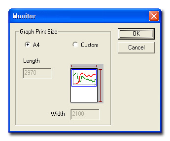
Print Graph Setting
If the dimensions of the printed graph do not correspond to the graph
on the monitor, it is possible to enter the width and length of the graph
manually. The user can modify the two Length and Width boxes by Selecting
the item CUSTOM.
Exit
Closes the application.
Connect
Connects the Monitor application to the instrument: if the Autodetect
function in Options >> Port Setting
is enabled, the serial port parameters are set automatically.
See the chapter Avvio di Monitor for
the connection details.
Disconnect
Disconnects the Monitor application from the instrument enabling the
use of the serial port for other applications.
New session
Deletes the data downloaded to the PC and opens a new measurement session.
As a precaution, the application asks if you wish to save the measurements
to a file.
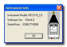
Inst. Info
Opens a window with the information for the instrument.
Monitor
Opens the window for the selection of the channel to be monitored using
the current settings.
To modify and display the parameters of the monitor function, start the
Setup. (See the details).
Instrument Setup
Opens the configuration page of the instrument connected to the PC. (See
the details).
Start Recording
Starts the recording of the data on the instrument using the current settings.
To modify and display the recording parameters, start the Setup. (See
the details).
Stop Recording
Ends the recording of the data (See the details).
Clear Instr. Mem.
Clears all the files contained in the instrument's memory.
The window to confirm the operation will appear:
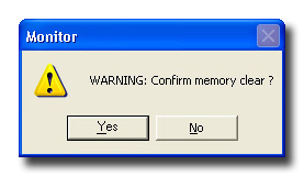
By pressing YES all recorded files are permanently removed.
The clearing is confirmed by the following window.
Note: the cleared files cannot be recovered.
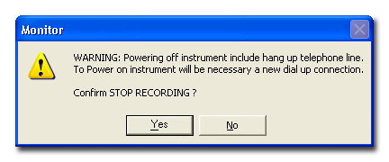
Instrument Power Off
Terminates the acquisition operations in progress and turns the instrument
off. This function is particularly useful in case of remote
connection via modem in order to interrupt the communication. In this
case, to access the sound level meter, a new
connection is necessary.
Refresh monitor
This function refreshes the data flow which is being received during the
monitor. This function can be used in the slowest of PCs unable to keep
up with the data flow received, to restart after an interruption of the
reception.
Acquisition >> Start
Starts the acquisition of data from the instrument performing the same
function of the RUN/STOP/RESET button on the keyboard when the instrument
is in the STOP phase.
Acquisition >> Stop
Ends the measurement execution and sets the instrument to STOP mode, performing
the same function as the RUN/STOP/RESET button on the keyboard when the
instrument is in the measurement phase.
See also the chapter on Display Data
View Full Date-Time
Changes between absolute and relative date and time both in the graphs
and in the data tables.
(See the details in the relevant chapter).
View 3D Graph (Three-dimensional Spectrum)
Graphic form used for the visualization of three-variable
graphs: frequency, width and number of samples. It is applied to multiple
octave and third octave spectrum and to reverberation time measurements.
View UR level
On the graph a horizontal line corresponding to the Under Range level
can be seen, representing the lower limit of the measurement dynamic of
the instrument.
Instrument bar
It enables or disables the Instrument bar
Status bar
It enables or disables the Status bar
Copy to Clipboard
This command copies the current window to the Windows Clipboard as both
a graph or table and allows it to be pasted as an image in another application.
After selecting the menu item Copy to Clipboard, open the destination
application (editor, spreadsheet, graphic application, ...) and use the
Paste command (or Paste Special if available) to paste the clipboard's
contents.
Zoom +
Enlarges a previously selected area of the graph. By holding down the
left button of the mouse and moving the pointer over the graph you can
select the area to be enlarged. Once the area is selected, use Zoom+
(or the Apply Zoom button), to perform the enlargement. (See
the details).
In case an octave and third octave spectrum is displayed, after pressing
Zoom+ the following window appears:
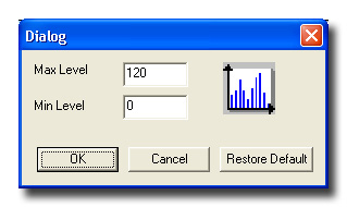
Max Level and Min Level represent the maximum and minimum level of the graph. The Restore Default button resets the standard default value levels.
Zoom -
Returns to the standard display for the SLM and History Profile graphs
and opens the window for the spectra described in the previous point.
Navigator
Opens the Spectrum Navigator (See the on line Help for DL5Viewer or DeltaLog5).
View E.L.Level >> E.L.Level 1987 (Isophonic
curves 1987)
Enables the drawing of isophonic curves in third octave spectrum according
to ISO 226/1987.
(See the paragraph Isophonic Curves ).
View E.L.Level >> E.L.Level 2003 (Isophonic
curves 2003)
Enables the drawing of isophonic curves in third octave spectrum according
to ISO 226/2003.
(See the paragraph Isophonic Curves ).
View Instr. Status
Recalls the window that resumes the current status of the sound level
meter. This page automatically appears when the application is connected
to the sound level meter (See the paragraph Monitor
Start up).
Scheduler
It opens the scheduler settings window for the Monitor function. Once
the settings are entered, press START to activate the scheduler.
For the details see the paragraph dedicated to the Scheduler.
View scheduler report
Displays the report saved together with the data file.
TheScheduler function records its own activity to a text file.
This file is saved with the data file, and when next opened, can be displayed
with this command. The function is disabled in the case where the scheduler
is continuous without intermediate pauses.
Port settings
Opens the dialog box to set or display the parameters of the serial communication
port. The function is only enabled when there is no instrument
connected. By checking the Autodetect option, the application sets
the port parameters automatically (recommended option).
For detailed information see the chapter dedicated to Monitor
Start up.
Electric calibration
Starts the electric calibration program for the sound level meter.
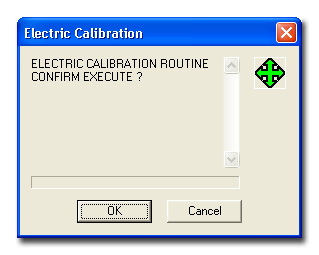
Press OK to start the program.
Wait for the conclusion of the procedure: a window appears asking for the new calibration data to be confirmed or not:
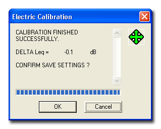
Press OK to save the new calibration, Cancel to exit without saving.
See the program details in the user's manual for the sound level meter.
Diagnostic Test
The diagnostic test is a program that verifies a series of the sound level
meter's parameters.
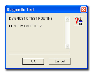
Press OK to start the program.
The program proceeds to verify the various points of the test and for each of them indicates a positive (OK) or negative (NO) result. The following summary page will appear at the end:
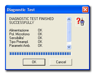
See the program details in the user's manual for the sound level meter.
Frequency check
The Frequency check program verifies frequency response of the
sound level meter on all the audio spectra by comparing it with the data
concerning the last periodic calibration available or with the manufacturer's
calibration. See the program details in the user's manual for the sound
level meter.
The following window appears when the menu item Frequency check is selected:
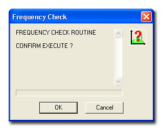
Press OK to start the test: before the scanning of the entire spectrum starts, the response at 1kHz to be used as a reference for the next steps is detected.
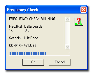
If this gave a positive result, press OK to continue. Then the octave frequency response is detected. The difference between the value detected and the reference value is indicated for each filter.
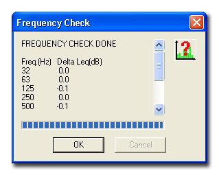
At the end of the check, if there is a clear difference between the two responses (high DeltaLeq), see the Troubleshooting guide in the User's manual.
Monitor module Info
Information on the software version.
To speed up the use of the system, some operations accessible trough the menus are also located on the command bar immediately beneath the main menu in the form of buttons.
|
|
File >>
Open |
|
|
File >>
Save as… |
|
|
Instrument >>
New Session |
|
|
Instrument >>
Connect |
|
|
Instrument >>
Disconnect |
| Instrument >> Monitor Opens the configuration window of the Monitor function. |
|
|
|
Instrument >>
Start Recording |
|
|
Instrument
>> Stop Recording |
|
|
Instrument
>> Instrument setup |
Tool
>> Scheduler |
|
|
|
Tool >> Zoom+ |
|
|
Tool >> Zoom- |
| |
View
>> View Full Date-Time |
| |
View >>
View 3DGraph |
| |
Tool
>> Copy to Clipboard |
|
|
File >>
Export to Excel (Export to Excel)
|
|
|
File >>
Print |
Upon connection a window may appear indicating a baud rate value lower than the maximum available:

A low baud rate value usually results in a useless slowing down of the data transfer from the sound level meter to the PC. Consequently, when no connection problems are present, it is recommended that maximum baud rate possible on the instrument be set (equal to 56700 baud) and to reconnect.
If the application does not connect, check the following:
Check that there are no active applications using the serial ports (e.g. Hyperterminal) on your computer. In such case close these applications and retry.
Ensure the serial cable used is the correct one: for direct connection of the sound level meter to the PC use the HD2110/CSNM cable; for the connection of the sound level meter to the modem use the HD2110/CSM cable. Do not use any extension without consulting with Delta Ohm.
For remote connection, use of the modem models tested by Delta Ohm is preferable. See the description in chapter Monitor Start up.
If there are other devices connected to other serial ports, they may interfere with the Monitor application. In this case it is better to set the parameters of the serial port manually by selecting the Port settings item in the Options menu.
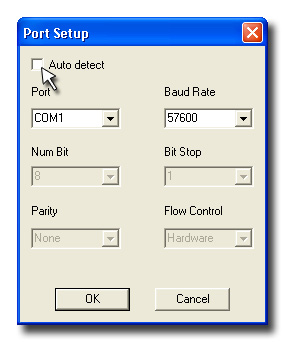
The serial port configuration window opens: by deselecting the Auto detect item the port to which the instrument is connected and the baud rate can be selected.
In this case, in order for the serial communication to work, the baud rate value set in the Port Setting window and that set on the instrument need to be the same.
How to set the baud rate on the instrument:
Open the menu using the MENU button: select the Instrument item and then the submenu Input/Output. The parameter to be modified is indicated as RS232 Baudrate. (Please see the detailed information on the instrument manual).
To minimize data transfer times, it is recommended that the maximum baud rate is set to 57600.
If you encounter problems during printing, try to
update the printer driver by downloading it from the manufacturer's website.
Using the File >> Print Graph Setting
command you can modify the printed image.
Use the Copy to clipboard function to
copy the current window and paste it in an other application: for example,
to print a graph copy and paste it into Windows Paint and try printing
it from this application.